Design Multi-Level Allocation Effect Using VisQuant

1. Top-Down Multi-Level (TDML) Decisions

The intent of this article is to demonstrate the early feature of VisQuant and collect your valuable feedback. The goal is to create a workflow that computes the top-down asset allocation effect. The top-down attribution model is used when the plan sponsor follows a top-down investment process. I will draft a detailed interpretation of the top-down versus bottom-up attribution model in future articles.

Before constructing the workflow, let’s define the mathematical frameworks for the asset allocation model (more details can be found in Bacon, C.R.[1]):

Unlike the bottom-up attribution model or single-level top-down attribution model, notice the benchmark weight notation $\widetilde{w}_i^B$, calculation of lower level asset allocation effects in TDML applied a trick to re-weight benchmark weight so that higher level benchmark weight becomes identical to the higher level portfolio weight.

With this adjustment on lower level benchmark weight, higher level asset allocation decision effect is isolated and does not spill over to lower level asset allocation decision. This calculation process is recursively applied to lower levels.

In VisQuant’s top-down attribution model, the user is allowed to construct an unlimited level of decision levels.

2. Basic Example and Using Prebuild Widget

Let’s apply this to a basic example:

A sample portfolio contains global allocation decisions to two counties (the US and Japan) and invested in both equities and bonds in each country. The long-term goal is built into the asset mix and set as the portfolio’s benchmark. The decision levels are as follows:

1. The fund’s committee/board makes a global allocation decision on overweight/underweight in the US and Japan. (i.e. $r_1^{AA}$)
2. An economist/strategist decides how the total assets in each country should be separated between equities and bonds, and makes allocation decisions in terms of relative exposures in each asset class. (i.e. $r_2^{AA}$)
3. Fund managers of each asset class take care of stock picking.

The fund structure is set up in VisQuant as shown below:

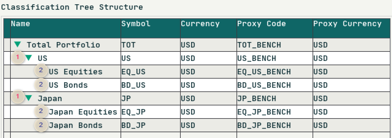
The example weights and one month returns of Sep-2017 is shown in the table below:

The sample portfolio can be attributed using the pre-packaged component widget Brinson (Multi-Period) to get results almost instantly:

From the resulting attribution analysis table shown above, the sample portfolio underperformed the benchmark by $18bps$ during the month. The first level country allocation decision(i.e. $r_1^{AA}$) added $14bps$, the asset class level decision($r_2^{AA}$) is attributed $-2bps$:

Let’s validate the second-level allocation effect for Japan Equities as an example. The new, rescaled benchmark weight using formula (2) for Japan Equities is shown below:

Applying formula (1) The second level asset allocation effect for Japan Equities is:

which is the same as the result from the component widget Brinson (Multi-Period).

3. Calculate Asset Allocation Effect - The Hard Way

Can I calculate the allocation effect using basic components? Absolutely, one of the key features of VisQuant is to help the users visually design their proprietary calculations.

3.1 Compute Adjusted Benchmark Weights

We can first start by importing and normalizing the sample portfolio and benchmark weights. Let’s implement the adjusted benchmark weights as formula (2) using Time Series Operations components as below:

The first step ( 1 shown above) is to compute the ratio of parent group between portfolio and benchmark, i.e. $\frac{w_S^P}{w_S^B}$. We supply the Time Series Operations component with the normalized portfolio and benchmark weights, Division operator allows you to calculate the ratio of the two weights.

We have not finished the calculation of the first step. Because the adjusted weight is calculated from multiplication of lower level weight with higher level weight ratio. Therefore, we need to shift the ratio down one level with option Copy Parent Value as shown below:

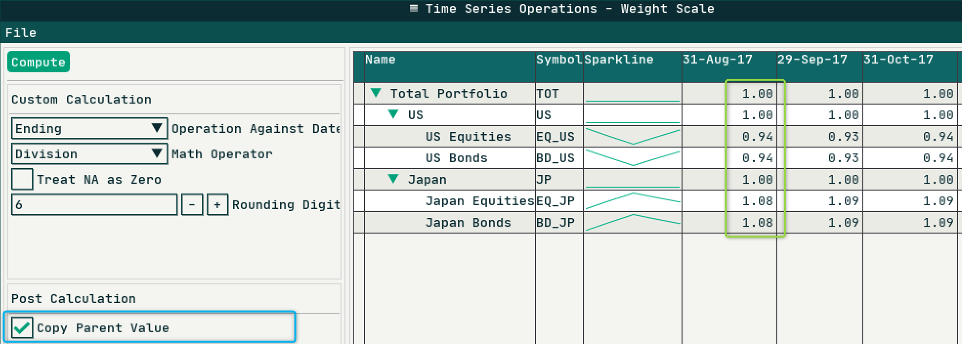
We can now implement second step (2 shown above) using Multiplication Operator from a new Time Series Operations component. Notice the Japan Equities adjusted weights $8.13\%$ shown below, it matches the manual calculation example that I demonstrated previously.

3.2 Compute Benchmark Relative Return Against Group

Let’s using import benchmark returns and apply Weighted Average component to calculate group and total level performance. The output of Normalization component for Benchmark Weight can be reused as input of Weighted Average component. The newly added Weighted Average component is shown below:

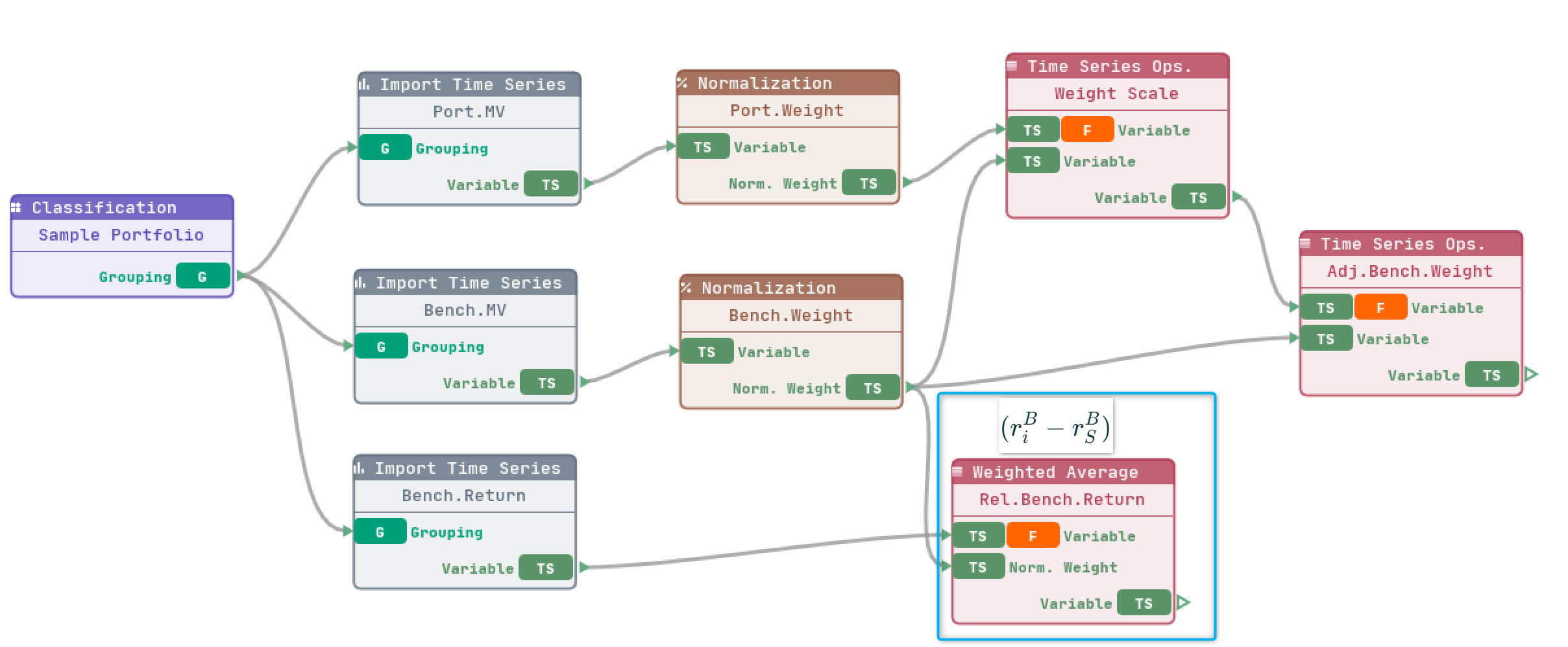
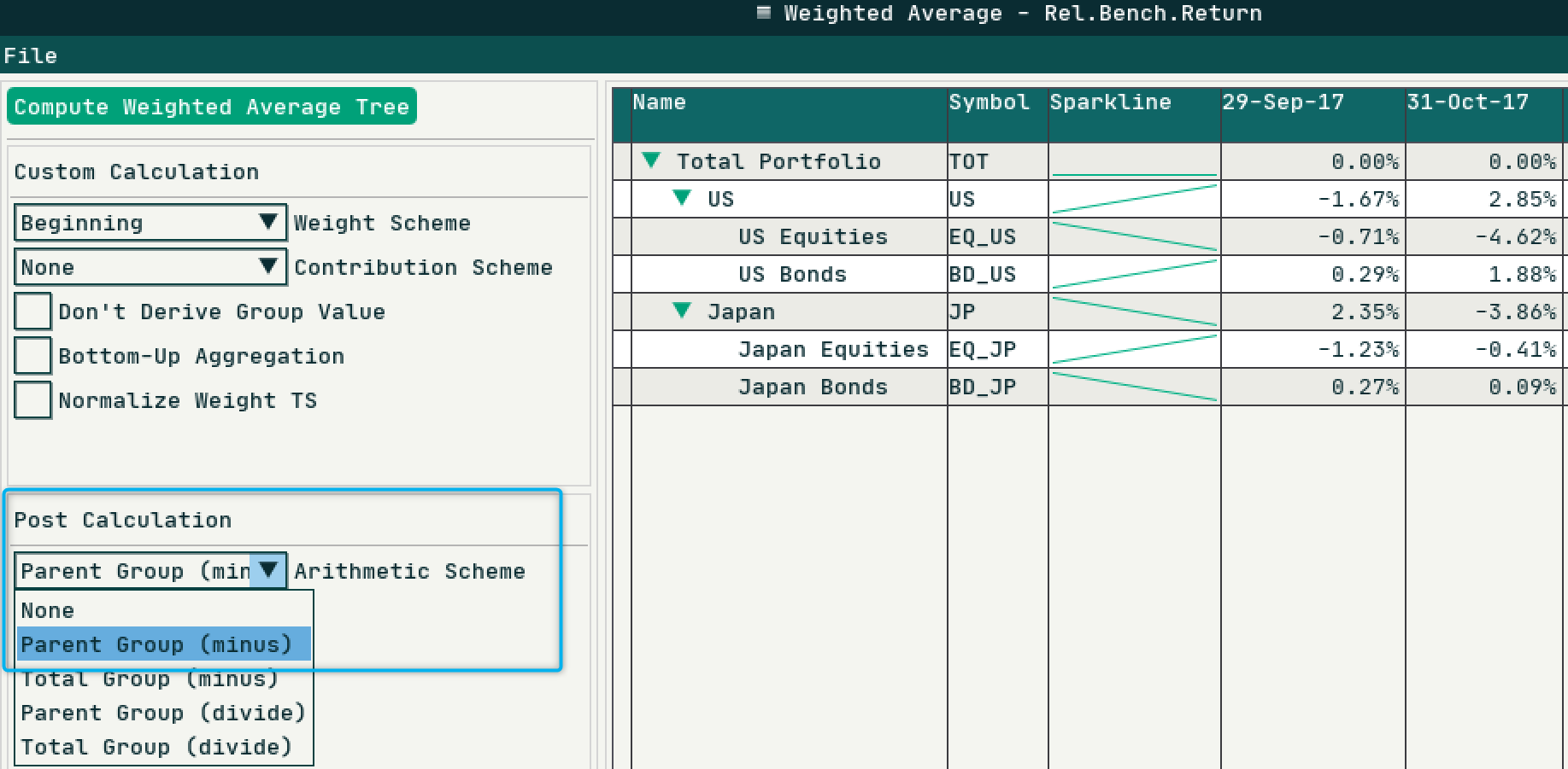
Using Weighted Average component, we can easily calculate performance for higher level segments $r_S^B$, but there is more than that. To calculate relative benchmark performance against higher level grouping $r_i^B-r_S^B$, simply select Parent Group (minus) as post arithmetic calculation scheme, the child level performance will be subtracted with parent level performance for all levels. The results are shown below:

3.3 Two More Arithmetic Operators To Get Allocation Effect

Finally, if you got this far, it will be easy for you to compute the final top-down allocation effect using two more component widgets:

1. One Time Series Opration to compute relative benchmark weights, i.e. $w_i^P-\widetilde{w}_i^B$

2. Another Weighted Average to multiply relative weight with relative benchmark performance, i.e. $(w_i^P-\widetilde{w}_i^B)(r_i^B-r_S^B)$

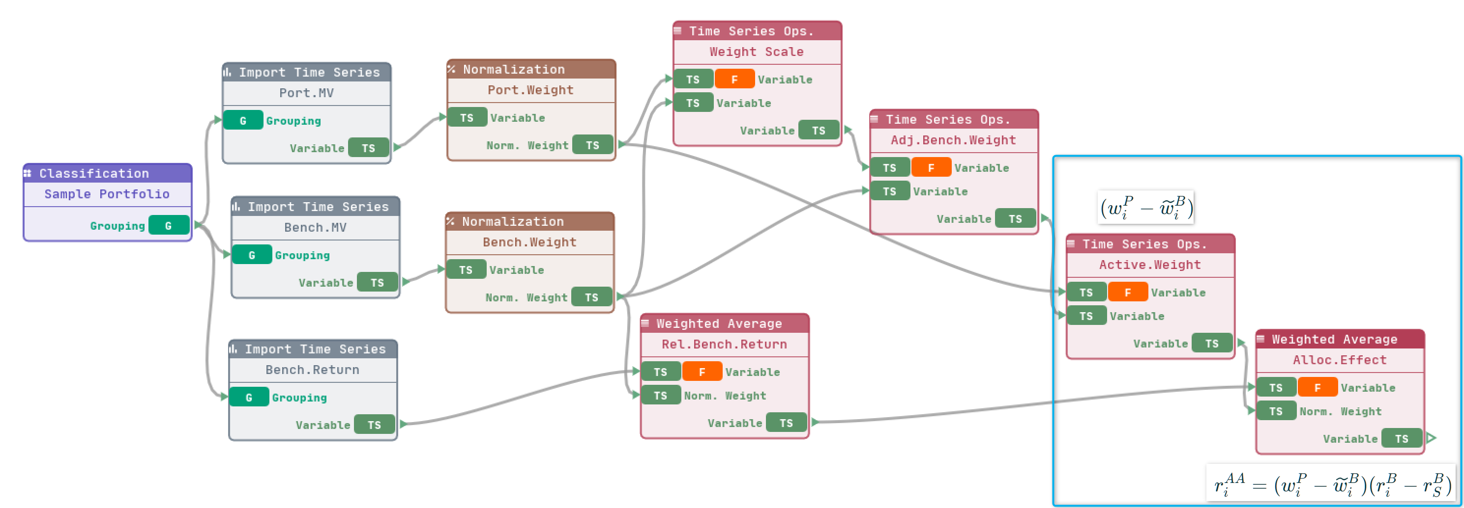
The final result produced by the above workflow is same as prebuild Brinson Multi-Period component widget:

4. Visual Programming Versus Prebuild Component Widget

What are the benefits of visual programming in the context of portfolio analytics? The main advantages are:

• you could build a lot of custom analytics,
• minimize your usage of excel and human error,
• and your data processing logic is more clear and transparent.

For example, constructing your proprietary quantitative strategies using VisQuant’s workflow. You could bring along your quantitative workflow for transparent discussion rather than talking with a black box.

Not everything gains a competitive advantage from being constructed as a workflow! There could have analytics calculations dependent on many other preconditions/settings; There are computation processes that are not easy to generalize as a component widget; You may have a huge graph after designing your process as a workflow that is hard to comprehend and so on.

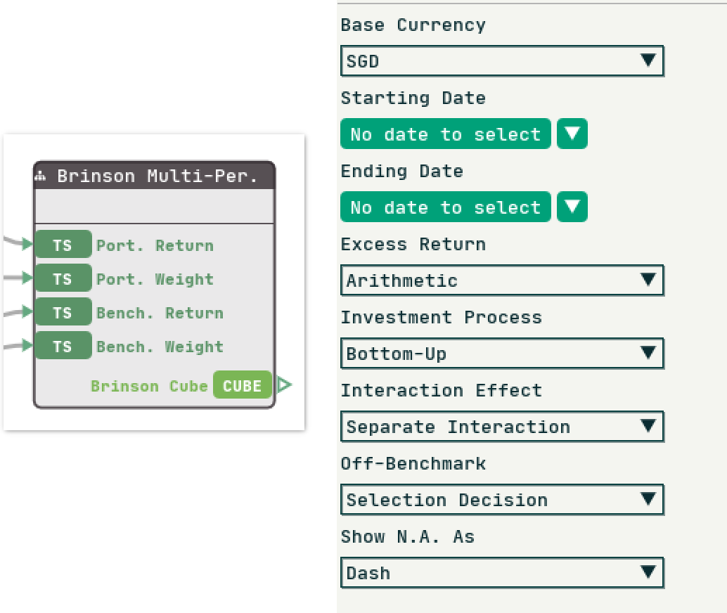
In those situations, it would be better to construct a prebuild component widget to bundle complex logic together. For example, Brinson Multi-Period is constructed to contain commonly used models and settings:

• Excess return model: Geometric or Arithmetic
• Investment process: Top-down or Bottom-up
• Off-benchmark treatment: Selection decision or Allocation decision
• and more

Feedback

That was a quick demonstration on key feature of VisQuant. I plan to provide more updates on functionalities and improvements in future posts. Meanwhile, I invite you to submit your recommendations or feedbacks through the VisQuant Public.

References

[1]: Bacon, C. (2008). Practical portfolio performance measurement and attribution, 2nd edition. Wiley Finance.